This article is the first among the series of planned articles which focuses on understanding and implementing the concepts of deep learning and artificial intelligence.
“Artificial Intelligence is the new electricity. Similar to how electricity revolutionized a number of industries about hundred years ago, artificial Intelligence will transform and revolutionize different industries” - Andrew NG
Artificial Intelligence and Deep Learning are becoming one of the most important components of modern day businesses. A large number of smart and intelligent systems are regularly built to solve the use cases that were earlier thought to be complex to solve. Some examples include automatic speech recognition in smartphones, conversation chatbots, image classification and clustering in search engines, natural language generation and understanding.
At a broader level, Artificial Intelligence and Deep Learning aims to create intelligent machines. However at a much deeper level, it comprises of Mathematical relationships, sophisticated optimization algorithms, and models that generate intelligence in the form of predictions, segmentations, clustering, forecasting, classifications etc.
The building blocks of every Artificial Intelligence and Deep Learning models are Neural Networks. In this article, we will understand everything about the neural networks and the science behind them.
Contents:
- Introduction of Neural Networks
- Single Processing Units - Neurons
- Activation Functions
- Forward Propagation
- Back Propagation
Introduction of Neural Networks
A neural network is a mathematical model that is designed to behave similar to biological neurons and nervous system. These models are used to recognize complex patterns and relationships that exists within a labelled data. A labelled dataset contains two types of variables - predictors (some columns which are used as independent features in the model) and target (some features which are treated as dependent variables of the model).
1. Employees data containing their information such as age, gender, experience, skills and labelled with their salary amount (example of numerical data)
2. Tweets labelled as positive, negative or neutral (example of text data)
3. Images of Animals labelled with Name of the Animal (example of image data)
4. Audios of Music labelled with the Genere of the Music (example of audio data)
The core structure of a Neural Network model is comprised of a large number of simple processing nodes which are interconnected and organized in different layers. An individual node in a layer is connected to several other nodes in the previous and the next layer. The inputs form one layer are received and processed to generate the output which is passed to the next layer.
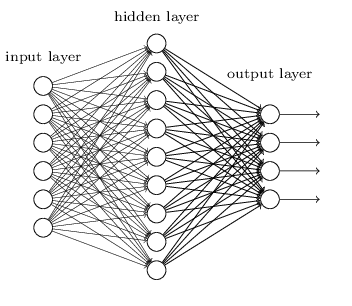
The first layer of this architecture is often named as input layer which accepts the inputs, the last layer is named as the output layer which produces the output and every other layer between input and output layer is named is hidden layers. Let us now understand the working of neural networks.
Single Processing Units - NeuronA neuron is the smallest unit in a neural network. It accepts various inputs, applies an function and computes the output.
Each incoming connection corresponds to different inputs to a node, To each of its connections, the node assigns a number known as a “weight”. The weight of every input variable signifies the importance or the priority of that variable among all other variables. For different values of input variables, the node multiplies the value with its associated weight and adds the resulting products together. It also add another term called “bias” which helps the learning function to adjust to left or right. This summed number is then passed through an activation function (described in next section) which maps the inputs to the target output values.
Lets understand this through an example. Take a situation in which the you want to purchase a new house and you will make the decision based upon the following factors in the order of their priority.
- Cost of the Property
- Square Feet Area
- Construction Year
- Availability of Security Systems
- Nearby Amenities
- Climate Factors in the Locality
- Crime Rate in the Locality
The best way to formalize the decision making based in this situation is to formulate a mathematical equation with:
- Every factor is represented as x1, x2, x3, …
- Every factor’s priority is represented as the weight: w1, w2, w3
- Node Input is represented as the weighted sum of factors and their weights (Z)
- Node Output is represented as the value of mapping function g (Z)
- Inputs: x1,x2, x3, …
- Weights: w1, w2, w3, …
- Node Bias term: “b”
- Node Input (Z) = w1*x1 + w2*x2 + w3*x3 + w4*x4 + … + w7*x7 + b
- Node Output (A) = g (Z)
Here the function “g” is known as Activation Function. Let’s understand how these activation function works.
Activation Functions - Applying Non Linear Transformations
The main goal of an activation function is to apply non-linear transformation on input to map it to output. For example a linear combination of 7 variables related to house are mapped into two target output classes: “Buy the Property” and “Do not buy the Property”.
The decision boundary of the output can be given by a threshold value. If the generated value is below a threshold value, the node outputs 0, otherwise 1. The generated outputs (0, 1) belongs to the decision. If A is the generated output (Activation), and “b” is the threshold, In our example, if weighted sum of inputs and their weights comes out to be greater than “b” you will buy the property otherwise not. ie.
if A > 0, then interpretation = “buy house”
else A < 0, then interpretation = “do not buy”
WX + b > 0, 1(“buy house”)
WX + b < 0, 0(“do not buy”)
This is the basic equation of the activation function which is applied at each neuron. In the above example, we have applied Step Function as the activation function.
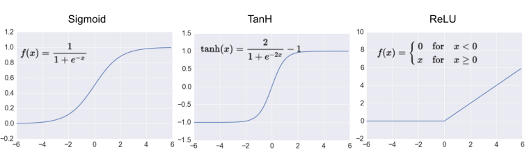
There are other choices of non linear activation functions such as relu, sigmoid, tanh:
Forward Propagation
Neural Network model goes through process called forward propagation in which it forward propagate the inputs and their activations through the layers to get the final output. The computation steps involved are:
Z = W*X + b
A = g(Z)
- g is the activation function
- A is the predicted output using the input variables X.
- W is the weight matrix
- B is the bias matrix
To optimize the weights and bias matrices used in the neural network, the model computes the error in the output and makes small changes in the values. These changes are made so that the overall error can be reduced. This process of error computation and weights optimization is represented in functions called loss function and cost function.
Error Computation: Loss Function and Cost Function
Loss function measures the error in the prediction and the actual value. One simplistic loss function is the difference of actual value and predicted value.
Loss = Y - A
Y = Actual Value, A = Predicted Value
Cost function computes the summation of loss function values for every training data example.
Cost Function = Summation (Loss Function)
Backpropagation: Minimizing the Cost Function using Gradient Descent
The final step is to minimize the error term (cost function) and obtain the optimal values of weights and bias terms. A neural net model does this through a process called backpropagation using gradient descent.
In this process, it computes the error of the final layer, back passes it to the previous layer. The previous layer associated weights and biases are adjusted to tackle the error. The values of weights and bias are updated using the process called gradient descent. In this algorithm, the derivative of error in the final layer is computed with respect to each weight. This error derivative is then used to find the derivative of weights and bias which are then subtracted from the original values to get the updated new values.
Then, the model again forward propagate to compute the new error with new weights and then will backward propagate to update the weights again. This will go on until some minima for error value is achieved. The process is repeated several times to achieve the minimum error term. This process is also termed as training. During training, the weights and thresholds are continually adjusted until training data with the same labels consistently yield similar outputs.
Recap
To train a neural network model, following steps are implemented.
1. Design the architecture of a neural network model with number of layers, number of neurons in each layer, activation functions etc.
2. For every training example in the input data, compute the activations using activation functions.
3. Forward propagate the activations through the input layers to hidden layers to output layer
4. Compute the error of the final layer using Loss Function
5. Compute the sum of errors for every training example in the input data using Cost Function
6. Backpropagate the error to the previous layers and compute the derivative of error with respect to weights and bias parameters.
7. Using Gradient Descent algorithm subtract the weight and bias derivative terms from the original values.
8. Perform this operation for a large number of iterations (epochs) to obtain a stable neural network model.
In this article, we discussed the overall working of a neural network model. In the next article I will talk about implementing a neural network model in python. Feel free to share your comments. In the next part, we will discuss about how to implement a neural network in python.