In the last article about neural networks, I discussed the topics - perceptron, sigmoid neurons, architecture of a neural network and learning of a neural network - gradient descent. We also applied a back propagation algorithm using Stochastic gradient descent in order to train the network. In this article, I will discuss about backpropagation algorithm in detail.
Quick Recap - We had built a neural network with one hidden layer, using sigmoid activation functions. Each training example (input feature vectors) is passed as input to the network. These are feedforward in the network using non linear sigmoid activation function. Output at each node is given as sigmoid function of (w. a’ + b), where w is the weight, a’ is the activation from previous layer and b is the bias vector. Now, the task is to train the network, hence the error term / loss / cost function is calculated using stochastic gradient descent (SGD) is used with backpropagation algorithm. In language of machine learning, training means the process of tuning the weights and bias variables so that error term is minimized.
What is Backpropagation Algorithm ?
In backpropagation algorithm, gradient of the cost function (delta change in cost) is calculated at the final layer. This gradient (error) is back passed to previous layers, by which changes are made in current weights and biases (delta weights and delta biases are subtracted from original values). This process is iteratively performed until cost function reaches the minimum value. The results of backpropagation algorithms can be grasped with the fact that every delta change made at the node level, affects the output of the network.
How Backpropagation Algorithms work ?
Since there are multiple cost functions, which are calculated for every training example. Final cost function can be computed as the average of all individual cost functions. Backpropagation works using four basic mathematical equations:
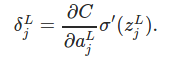
L: Final output layer
C: Final Cost Function
the above equation states that the error of final layer can be computed using derivative of cost with respect of final activation as computed in output layer. The term signifies that how fast cost function changes with respect to the activations. This term is multiplied with sigmoid prime of input vectors of final layer which signifies, how fast an activation is changing due to change in inputs.
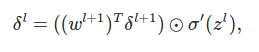
The above equation states that the error of a layer can be written in terms of error of next layer. This generates back passes. The error of a layer is hence weight matrix of next layer times error of the layer, this is then multiplied using hadamard product with sigmoid prime of current layer inputs (current activation)

Bias parameters can be computed using error of the layer
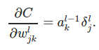
Weight parameters can be computed using error of the layer. Hence, the complete backpropagation can be summed up as:
1. Input the x - training example
2. Feedforward the activations through each layer, and compute final activation.
input terms: z = w.a’ + b & activation function: sigmoid (z)
3. Calculate the error term of final layer: delta L, using equation , which can also be written as ∇aC ⊙ σ′(zL)
4. Backpropagate the error using equation [2] δl=((wl+1)Tδl+1)⊙σ′(zl)
5. Adjust weights and bias, using equation [3] and [4]
The complete code is available here, Here